List Comprehensions in Python

When you need to do something involving a list in Python, either process an existing list or create a new list, there’s a kind of shorthand that can be used to do this in a single line between square brackets, called ‘List Comprehension’. Think of it as For loops within list brackets, with or without conditionals.

# given a list
casual_names = ['alec','jude','malcolm']

capitalized_names = [name.title() for name in casual_names]

You can add a conditional statement. For example, square all the even integers in a given range:

squares = [x**2 for x in range(16) if x % 2 == 0]

You can use if else statements, but they have to appear before the for. Convert positive and negative reviews to integers:

# for a list of reviews
reviews = ['positive','negative','positive']

# encode them as 1's and 0's
encoded_reviews = [1 if r == "positive" else 0 for r in reviews]

Snakemake Basics

Make files are a great way to get things done efficiently, if you know what they are and they make sense to you. My entry into makefiles started when I took C programming in the late 80’s. You would write code in C, then use a Makefile to turn that code into an executable program. Since it takes several intermediate steps and creation of different kinds of files along the way, a Makefile manages all these steps using recipes laid out in blocks. The blocks are designed to create output files from input files. You specify the names of the output files, and the names of the input files, and a set of rules for how to use one to create the other.

Snakemake is this same idea, implemented through python. Here’s a simple example.

all:
    alignment.bam         # We have to populate this part with the files we want to create

align:
    input:
        input.fastq       # [FileSystem] Does this file exist?
                          # Is there some rule to create it?
    output:
        alignment.bam     # Does this part match any part of "all"?
                          # [FileSystem] Does this file already exist?
    shell:
        bowtie input.fastq | samtools > alignment.bam

Generate Random Integers in Python

Getting random integers in Python

# import the function
from random import randint

# set your parameters
howmany = 10
min = 0
max = 100

# use a list comprehension to fill an array
rand_ints = [randint(min,max) for _ in range(howmany)]

Seems kinds of bulky, but you specify how many numbers you would like, what range to draw them from, and then call the radint() function over and over again until you have the numbers you need, using a for loop with a throaway variable “_”.

But there’s a few ways to do this! If you have NumPy installed, it has a similar function for generating random integers, and the lines of code above, can be reduced to just two: import the library, call the function.

from numpy.random import randint

randint(0,100,10)

The result is as follows:

array([42, 99, 30, 94, 60, 90,  7, 31, 91, 11])

Both of these methods would usually be preceded by a call to “seed” the random number generator, so that you can set a reproducible starting point for random number generation. The function has the same name in each library, and calling seed for one does not set the seed for the other. But that’s more than you need to know for now.

Recording and Editing Lectures with Zoom and Shotcut

It’s Fall. School is starting, but we’re in the middle of a world wide viral pandemic so most students are not going to be present in person for the lectures you’d like to deliver to them. During the summer I attended many conferences that had pre-recorded talks. HOPE2020 was particularly impressive in terms of the quality of the presentations. How did they do it? I think most people used zoom, but I’m not quite sure how they actually did it, especially if any editing was involved. I have a bunch of lectures to prepare, so I figured I’d share my experience.

A lot of people are teaching and presenting remotely these days. What platform should you use to record a lecture? Zoom is a freely available, popular, and ubiquitous platform with many nice features. Zoom can be used to record a presentation, allowing you to share your computer screen, while simultaneously allowing you to appear in the presentation with picture in picture mode if you choose.

The only thing you need to record a lecture is a Zoom account, the Zoom software, and a desktop or laptop computer. Recording doesn’t currently work with phones or tablets.

To record a lecture, open the Zoom software, start a meeting with yourself, and then push record. There are options for sharing your screen, and for either pausing or stopping the recording. The difference between pause and stop has to do with the number of output files at the end. Using Pause will preserve everything in one video file, whereas using Stop to halt recording will produce a separate video file (serially numbered) for each time the recording was stopped.

On my mac, Zoom has been recording at a resolution of 1440 x 900 at 25 fps, and roughly 1 MB per 15 seconds of video. So a 45 minute lecture may come out as 180 MB or so. The result of a recorded lecture is an mp4 file with video and audio, as well as a separate file containing just the audio.

If you need to edit the video, or splice together pieces of video, this can be a bit tricky as many programs take in the video in one format, but then change the format or resolution upon export. For instance I tried making a simple edit in Quicktime, but then the format changed to MOV. So I tried taking it into iMovie, but the only available export formats all had 60 fps, so the video ballooned from 160 MB to 2 GB.

Luckily I found a free, open source video editing program called shotcut. It runs on all platforms. I was able to splice together a few clips very easily. It preserved the input resolution for export. So it spit out exactly what I put in: 1440 x 900 at 25 fps, and the final size of my video matched what I would have had coming directly out of Zoom.

I was able to use shotcut seemlessly after watching 10 minutes of a tutorial on youtube. Basically, import clips, drop them into the time line, edit them in the timeline by splitting the clips at the play head (s key) and removing the portions I didn’t want, then exporting the finished product.
Python Dictionaries

A dictionary in python is an associative array. This means you can use it to hold an array of things, and associate names, or keys with those things so they can be retrieved. Dictionaries use curly brackets in their declaration:

my_dict = {'pi': 3.14, 'e': 2.71, 'gravityAccel': 9.8}

to access a given element, you use square brackets on the key:

my_dict['pi']

You can process a dictionary using a for loop and the “in” keyword:

for key in my_dict:
  print(key, "->", my_dict[key])

You can also loop through the keys and values together, using the items() method on your dictionary:

for key, value in my_dict.items():
  print(key, "->", value)

The elements of a dictionary can also be accessed by methods:

dictionary_values = my_dict.values()
dictionary_keys = my_dict.keys()

Quickly examine just the first 5 items in your dictionary, take a slice of a list:

list(my_dict.items())[:5]

Comprehensions are often used for processing dictionaries. For instance, reversing the keys and values:

my_reverse_dict = {v: k for k, v in my_dict.items()}

That’s a lot – creating a new dictionary, looping through the old dictionary, and reversing the keys and values all in one line.

And this can be combined with conditional statements such as “if”:

my_filtered_reverse_dict = {v: k for k, v in my_dict.items() if v > 3}

Simple Life Grid

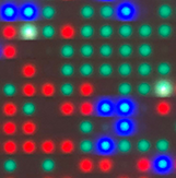
In 2016 I bought a 32×32 RGB LED Matrix Panel (6mm Pitch – distance between LEDs) from Adafruit.com because I wanted to build a project based on Conway’s cellular automata game. I had seen a similar idea in a booklet of Raspberry Pi projects that was slim on details but mentioned enough that I could find a code repository describing a simple simulation involving 2 species that would cohabitate the grid. It also linked to a C library that could drive the grid (as did the adafruit website). Adafruit makes and sells a HAT (Hardware Attached on Top) to make it easy to bridge the Pi to the LED grid.

This is where things got a little confusing for me. I’m good at soldering and assembly, so getting everything together was no problem. The tutorials at adafruit are easy to follow. I downloaded the rpi-rgb-led-matrix library, and had the matrix going in no time. It was fun to play with the functions in the example code, and write a routine to get a single spot to run around the screen changing directions randomly. Explaining C code, and make files to my 8 year old son, and watching him get excited about edit, make, run, was very satisfying. The only downside of having young kids – when you get stuck, your project can sit indefinitely.

And that’s what happened. Trying to bridge the gap between ferrithemaker’s lifebox code and the LED grid, was tough. I was never able to figure it out. I tried the code out of the box, no luck. I tried recoding GPIO pin identifiers to make sure they matched the adafruit HAT description. No luck. I scoured as many specs as I could find, and looked around for how the lifebox functions operate to control the LEDs. No luck.

Finally, since I had a working chunk of example C code from the hzeller distribution, I simply inserted the core of the lifebox grid into that, and replaced the drawing functions with those from the rpi-rgb-led-matrix library. Voila! It worked on my first compile!

Now that it’s working I can tweak the logic and add my on rules and interactions. Maybe hook it up to other inputs. For instance, it would be nice to model the plant behavior based on local weather – rain: more plants. No rain + heat: fewer plants. Maybe let the species eat each other. Find a way to add a mutant species every now and then. Alec’s 10 now, and my project is where I wanted it to be 2 years ago. But at least it’s progress!

Sample a BAM file

When working out a pipeline, especially those involving BAM files, I often find it useful to create some toy sample data to push through it, just to get it working. Most BAM files I use contain millions of reads and are often gigabytes in size. Using full size files can burn lots of time just to find out an error has occurred. Whereas using a file with only a few reads allows you to spot errors instantly. What if you simply want 1000 sequence reads from a BAM file? What is the easiest/quickest way to grab them? Use samtools view to grab reads and specify how many you’d like to keep using “head”.

samtools view -h in.bam | head -1000 | samtools view -b - > sample.bam

This won’t return exactly the number of reads you specify because the header of the BAM file will count as lines against the number you specify. The point of taking the small sample above it to not have to read through the whole file to get a few reads. However, another option which is generally more robust, but which will read though the whole file, is to sample the file. For instance, if you took every tenth read – you’d have a file that is approximately 20 times smaller, and there’s a samtools option for that:

samtools view -s 0.1 -b in.bam > out.bam

The -s option samples the file by taking only a fraction of the alignments, chosen randomly. The -b option in the command above specifies that the output should be in BAM format.

Paste0

The paste() function in R is a nice way to concatenate sets of values together. Let’s say you need to make up some fake gene expression data to illustrate a heat map.

# use rnorm() to generate 100 random values to fill a matrix
gdat <- matrix(rnorm(100), nrow=10, ncol=10)

We use the rnorm() function to grab 100 random values from a Normal distribution, and place them into a matrix. If this matrix is supposed to represent gene expression values, typically the rows would represent genes, and the columns would represent samples or conditions. We can use the paste() function to create names for the rows and the columns.

# create 10 fake gene names to label the rows
rownames(gdat) <- paste("g", 1:10, sep="")
# create 10 fake sample names to label the columns
colnames(gdat) <- paste("s", 1:10, sep="")

# now we can draw a heat map that will have row and column labels
heatmap(gdat)

The paste function takes a series of arguments to be concatenated, as well as a separator for each concatenation event. This is good for many things such as creating file names from other values:

mutants <- c("sir1", "cen3", "rad51")
datafiles <- paste(mutants, "txt", sep=".")

Or for dynamically creating a plot label:

paste("number of genes detected:", NumberOfGenes)

The default separator for paste() is a space character. So in the example above, I left out the "sep" argument because a space character will be inserted by default. Whereas in the first example with the heat map I did not want spaces to occur in my fake gene and sample names, so I specified: sep="" to overide the default.

Once you start using paste(), you'll use it a lot, and more often than not I would say you want to concatenate things without a space, or any other character. So I often find myself typing: paste(a,b,sep=""). A short cut for this is a function called paste0()! The paste0() function is paste with no default seperator! I always forget about it, but if you can remember it will save you a little bit of typing and make your code more readable.

# create 10 fake gene and sample names
paste0("g", 1:10)
paste0("s", 1:10)

BED files into R

Sometimes BED files drive me nuts. They’re great for their simplicity in specifying a genomic feature, but can be difficult to work with across programs because only the first three columns are required (chromosome, start, end) and there are several ways to specify any number of remaining columns. Well, maybe not any number, but looking at the following names, tell me if clarity jumps from the page: BED, BED6, BED8, BED12, BED6+4, BED15, any others? Even the spec at UCSC doesn’t explain the conventions behinds those names.

Working with BED files in R is typically fairly easy. The rtracklayer library contains import/export functions for reading or creating bed files. For instance, reading a bed file into a GRanges object is as simple as:

library(rtracklayer)
foo <- import("myPeaks.bed")

However, when those BED files are produced by programs like MACS2 that muck around with some of the fields, then things break, and you have to start figuring out all those unwritten rules about BED files. Typical UCSC BED format has 12 columns. MACS2 produces a narrowPeak file described as BED6+4. The R help for the import() function states the problem explicitly, and offers a solution: …many tools and organizations have extended BED with additional columns. These are not officially valid BED files…To import one of the multitude of BEDX+Y formats, such as those used to distribute ENCODE data through UCSC (narrowPeaks, etc), specify the ‘extraCols’ argument to indicate the expected names and classes of the special columns.

Now the problem is simply that we don’t know which of the columns are standard and which are “special”, and none of the columns of a BED file are “named”, leaving this bit of help a little confusing. But we can make some good guesses, and it turns out they work.

The first 6 fields of the MACS2 narrowPeak file have the properties expected by import() and conform mostly to the UCSC standard (the 5th column is supposed to be an integer between 0 and 1000, but for MACS2 it is simply the -log10 transformed peak Q-Value multiplied by 10 and converted to an integer). But the remaining 4 fields DO NOT match what import() expects, and thus have to be explicitly specified. Thus to get our MACS2 results into R we can do something like the following:

# declare names and types for the extra BED columns
extraCols_narrowPeak <- c(FoldChange="numeric", pVal="numeric",
qVal="numeric", summit="integer")

# import our peak data
peaks <- import.bed("my_peaks.narrowPeak", extraCols=extraCols_narrowPeak)

The result is a GRanges object called “peaks” with meta columns named based on what you gave to extraCols.

biohacking 2008

HOPE is a unique experience. Not a colorful crowd, literally. Cargo shorts and black shirts, as if everyone knows the uniform. But while you’re there, you feel a sense of connection with those around you unlike any other conference I’ve attended. The commonality goes beyond interest in a single subject matter and has to do with plain raw curiosity and freedom. Including the freedom to just be yourself without having to worry so much about social graces or comfort. Showers and sleep are completely dispensable. The talks go from 9 AM to midnight. I’ve sat down at 9 AM and not moved until 6 PM, to slip outside and grab a slice of pizza and a cup of coffee, only to get back ASAP and sit in talks until 12, before ending up at Harry’s or Sally’s down the street with various members of the 2600 crowd, and then wandering back to the hotel mezzanine to ride a Segway or pick some locks in the lock picking village. People wander around at all hours. The sidewalk in front of the hotel penn is busy around the clock. It’s surreal to step outside at 3 AM and hang with a crowd of like-minded people, all taking a break, while people are shuffling along the sidewalk and the street vendors sell sticks of grilled chicken.
This particular conference was jam packed with adventure and odd convergences for me. Adam Savage was one of the keynote speakers. I used to work down the street from the Alameda air base where so many episodes of Mythbusters were filmed, and having left the bay area just as the show was getting started, watching it always made me feel like I was home from afar. Kevin Mitnick was also a featured speaker. I grew up reading about him, read several books in which he is one of the main characters, followed his travails along with the 2600 crew while he was in in jail , and because of that, decided to omit making a connection during my talk between the discoverer of a cool protein often used in biohacking and the person who led to his capture. I didn’t want to take the glow off the protein as I didn’t think the crowd would be too enamored. I was interviewed for a documentary on hacking. It will be interesting to see if it gets off the ground. I had a lot of great conversations with people, including Bernie S,  whose voices I had only heard on the radio while I worked in the lab at Berkeley. It’s an odd thing when you find yourself face to face with people you feel some familiarity with, because you hear their voices or follow their lives or work, yet you only see them in a bar for a couple of nights every two years.
On the last night after the closing ceremonies, a large portion of the crowd sticks around to stack chairs, disassemble the large lighting structures, wrap and package up all the audio visual gear. Cord wrangling can be quite a skill. Kudos to those who have a hex wrench built into their keychains. After everything was cleaned up, I found myself wandering through the streets with Bunnie and the rest of the crew looking for a place to eat. We walked West and settled at a Chinese place. Emanuel sat across from me. As the waitress was taking drink orders, most everyone ordered an “OB”. I was in the mood for a beer, but I didn’t want to break the cycle, and was intrigued at what a Jedi sounding drink might be. I was happy and somewhat giddy when the waitress placed an Oriental Beer in front of me. Years of listening to him on the radio and reading his editorials might have led me to believe that Emmanuel speaks eloquently all the time about interesting issues on a range of topics. But after days of sleep deprivation, and only a few days of chance encounters in bars or the HOPE mezzanine, there was more silence between us than I had hoped for. Eventually more and more people started showing up, and introductions were made, but I was among people who knew each other much more than anyone knew me. If nothing else, at least the turquoise blue badge chord gave me speaker cred.
My talk was on Saturday afternoon in the small room with the portable wall separating it from the large room. I think I was competing with Rambom. He gives the same talk every time. Three hours of all the ways he can find information about anyone because of the way people voluntarily give up information on themselves. My talk was really well received. I actually ran out of time and had to skip several slides at the end. Nonetheless, I was hoping I could do a sufficient job explaining that biology is a lot like executing programs encoded in a sequence of information, and via synthetic biology we can make new programs.
For now, at least, I know I can look forward to the next hope.